Mortality rates are typically provided in an abridged form, i.e., by age groups 0, ‘[1, 5]’, ‘[5, 10]’, ‘[10, 15]’, and so on. Some applications require a detailed (single) age description. Despite the enormous number of suggested techniques in the literature, only a few solutions provide good results at both younger and older ages. For example, the 6-term ‘Lagrange’ interpolation function is appropriate for mortality interpolation at younger ages (with irregular intervals), but not at older ages. The ‘Karup-King’ method, on the other hand, works well for older age groups but is not appropriate for younger ones. Shryock, Siegel, and Associates (1993) provide an in-depth description of the two methods mentioned.The Q2q package combines the two approaches, allowing for interpolation of mortality rates over all age groups. Each approach is implemented independently, and the resulting curves are merged at the age at which the two partial curves show the smallest 5-age averaged error.
You can install the released version of Q2q from CRAN with:
install.packages("Q2q", repos='http://cran.us.r-project.org')
#> Installation du package dans 'C:/Users/lenovo/AppData/Local/R/win-library/4.2'
#> (car 'lib' n'est pas spécifié)
#>
#>   Une version binaire est disponible mais la version du source est plus
#>   récente:
#>     binary source needs_compilation
#> Q2q  0.1.0  0.1.1             FALSE
#> installation du package source 'Q2q'
Before it can be used, the package needs to be called.
library(Q2q)The package Q2q provides two functions
getqxt() and getqx().
The getqxt() function allows interpolating age specific
mortality rates \(ASMRs\) starting from
an abridged mortality surface. An abridged mortality surface provides
the five ages mortality rates, usually noted as \(_nQ_{x,t}\), with \(x\) representing the age and \(t\) the year and \(n\) the length of the age interval which is
set to be \(5\) except for age \(0\) and the age group \(1-4\).
The primary output of the function is qxt, which is a
matrix of the age-specific death rates for a given age \(x\) and year \(t\). This matrix was the product of the
junction of two initial matrices, qxtl and
qxtk, that were produced using the Karup-King and Lagrange
methods, respectively. Additionally, these two matrices are given as
function outputs. Moreover, the junction age is given as a vector
jUnct_ages for every year \(t\). In addition, the function returns the
theoretical death matrix qxt and the survivorship matrix
lxt.
The getqx() function is a special case of
getqxt() with t=1.
getqx <- function(Qx,nag) {
                           getqxt(Qxt=Qx, nag, t=1)
}In order to assess the quality of the interpolated mortality rates,
two types of tests are included in the Q2q package: the
Fidelity Test and the Zero-One Test, which were implemented as “Unit
tests” in the package and can be used by users to validate their own
results. Both test were developed using the testthat
package and the test outcome come either as Test passed or
Test failed.
library(testthat)
#> Warning: le package 'testthat' a été compilé avec la version R 4.2.3
The Fidelity Test measure the likelihood between the original
five-years mortality rates (before interpolation), i.e.Qxt,
and those recalculated from the interpolated rates, i.e.,
Qxt_test. Good results suggest that the errors observed
between Qxt and Qxt_test to be below a well
defined ceiling at all ages. In our case, we defined the maximum
tolerated error at 0.005, which seems reasonable in the
case of five-age mortality rates.
The test can be implemented using the following code:
test_that("Fidelity test", {
 data("LT")
  Qxt = LT
  expect_equal(getqxt(Qxt, nag=nrow(Qxt), t=ncol(Qxt))$Qxt,getqxt(Qxt, nag=nrow(Qxt), t=ncol(Qxt))$Qxt_test ,tolerance=0.005)

  Qx = LT[, 11]
  expect_equal( getqx(Qx, nag=length(Qx))$Qxt, getqx(Qx, nag=length(Qx))$Qxt_test,tolerance=0.005)
   })
#> Test passed
The Zero-One Test aims to ensure that the interpolated
rates are all comprised between 0 and 1. Under specific circumstances, a
high fluctuation of five-age mortality rates (e.g. crude rates), the
interpolated rates can be situated outside the 0-1 interval. This test
aims at making sure that this is not the case. The following code can be
used to implement the test:
test_that("zero-one test", {
  data("LT")
  Qxt = LT
  q = getqxt(Qxt, nag=nrow(Qxt), t=ncol(Qxt))$qxt
  n = nrow(q)
  t = ncol(q)
  expect_true(all(q>0 & q<=1))

  Qx = LT[, 11]
  q = getqx(Qx, nag=length(Qx))$qx
  n = nrow(q)
  t = ncol(q)
  expect_true(all(q>0 & q<=1))
})
#> Test passedThe package comes with a dataset containing the Algerian mortality surface from 1977 to 2014, for males, by 5 ages groups. We use the provided dataset for the two first examples. Data from external sources (Japonese Mortality Database) are used in the two last examples.
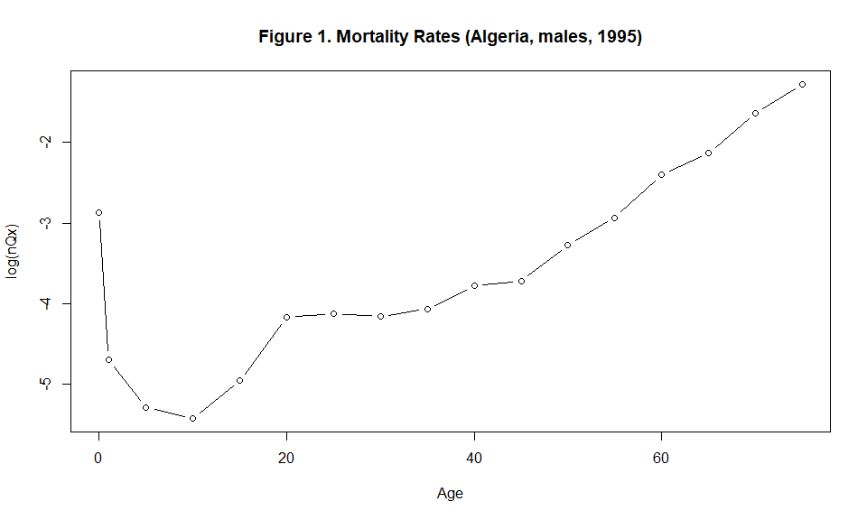
data("LT")Lets consider a case of an annual life table (Algeria, males, year 1995).
Ax <- LT[,18]
Ax
#>  [1] 0.056800000 0.009117897 0.005028889 0.004409076 0.007020197 0.015444855
#>  [7] 0.016129032 0.015607456 0.017109616 0.022745735 0.024106401 0.037843758
#> [13] 0.053243961 0.090569062 0.118830787 0.194365728 0.278272707
We plot the mortality curve.
plot(x=c(0,1, seq(5, (length(Ax)-2)*5, by=5)), y=log(Ax), type="b", xlab="Age", ylab="log(nQx)", main="Figure 1. Mortality Rates (Algeria, males, 1995)", cex=1 )
We interpolate q_{x,t} using getqx()
interpolated_curve <-getqx(Qx=Ax, nag=17)
str(interpolated_curve)
#> List of 8
#>  $ qx       : num [1:80, 1] 0.0568 0.00311 0.00247 0.00197 0.00159 ...
#>   ..- attr(*, "dimnames")=List of 2
#>   .. ..$ : chr [1:80] "0" "1" "2" "3" ...
#>   .. ..$ : NULL
#>  $ lx       : num [1:81, 1] 10000 9432 9403 9379 9361 ...
#>   ..- attr(*, "dimnames")=List of 2
#>   .. ..$ : chr [1:81] "0" "1" "2" "3" ...
#>   .. ..$ : NULL
#>  $ dx       : num [1:80, 1] 568 29.4 23.3 18.5 14.9 ...
#>   ..- attr(*, "dimnames")=List of 2
#>   .. ..$ : chr [1:80] "0" "1" "2" "3" ...
#>   .. ..$ : NULL
#>  $ qxk      : num [1:80, 1] 0.02178 0.01634 0.01209 0.00918 0.00771 ...
#>  $ qxl      : num [1:70, 1] 0.0568 0.00311 0.00247 0.00197 0.00159 ...
#>   ..- attr(*, "dimnames")=List of 2
#>   .. ..$ : chr [1:70] "0" "1" "2" "3" ...
#>   .. ..$ : NULL
#>  $ junct_age: num 44
#>  $ Qxt      : num [1:17, 1] 0.0568 0.00912 0.00503 0.00441 0.00702 ...
#>   ..- attr(*, "dimnames")=List of 2
#>   .. ..$ : chr [1:17] "0" "1" "5" "10" ...
#>   .. ..$ : NULL
#>  $ Qxt_test : num [1:17, 1] 0.0568 0.00912 0.00503 0.00441 0.00702 ...
#>   ..- attr(*, "dimnames")=List of 2
#>   .. ..$ : chr [1:17] "0" "1" "5" "10" ...
#>   .. ..$ : NULL
We plot the interpolated mortality curve using
plot()
plot(x=c(0:79), y=log(interpolated_curve$qx), type="b", pch=19, xlab="Age", ylab="log(qx)", main="Figure 2. Interpolated Mortality Rates (Algeria, males, 1995)", cex=0.75)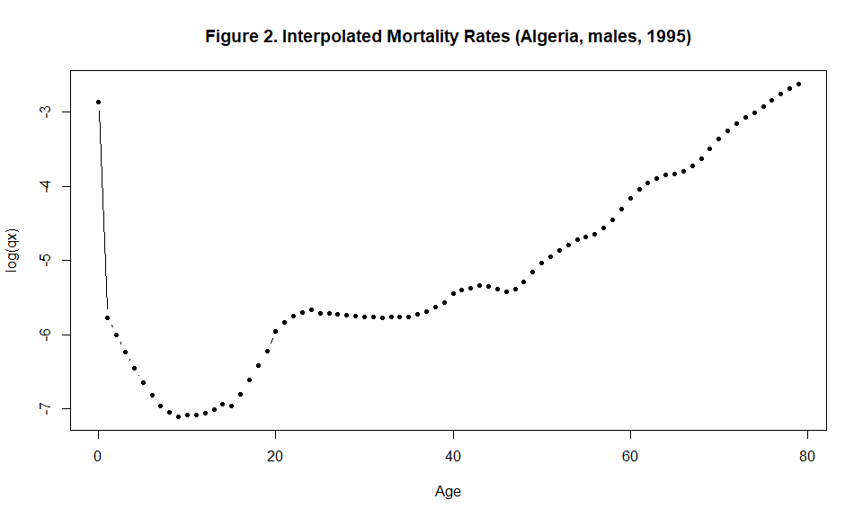
plot(x=c(5:79), y=log(interpolated_curve$qxk[6:80]), type="l", lwd=5, pch=1,xlab="Age", ylab="log(qx)", main="Figure 3. Interpolated Mortality Rates (Algeria, males, 1995) - Junction age", xlim=c(0,80), col="gray")
lines(x=c(0:69), y=log(interpolated_curve$qxl), lwd=2)
lines(x=rep(interpolated_curve$junct_age, 2), y=c(min(log(interpolated_curve$qxl)),max(log(interpolated_curve$qxk))), lty=2, lwd=1.25, col="red")
legend(x=2, y=-3, c("Lagrange Method", "Karup-King Method", "Junction age"), lty=c(1,1,2), col=c("black", "gray", "red"), lwd=c(2,5,2))
We validate the obtained results using the fidelity test and the Zero-One test.
test_that("Fidelity test", {
 # data("LT")
  Qx = LT[, 18]
  expect_equal( getqx(Qx, nag=length(Qx))$Qxt, getqx(Qx, nag=length(Qx))$Qxt_test,tolerance=0.005)
   })
#> Test passed

test_that("zero-one test", {
 # data("LT")
  Qx = LT[, 18]
  q = getqx(Qx, nag=length(Qx))$qx
  n = nrow(q)
  t = ncol(q)
  expect_true(all(q>0 & q<=1))
})
#> Test passedLets consider the following mortality surface with a dimension of 17 (age groups) by 38 (calendar years), the Algerian mortality surface from 1977 to 2014 for males.
Bxt <- LT
head(Bxt[  ,1:5 ])
#>         X1977      X1978      X1979       X1980       X1981
#> 0  0.12771000 0.11457000 0.10983285 0.107010000 0.101360000
#> 1  0.05712550 0.04550331 0.05024614 0.053628820 0.050487403
#> 5  0.01737471 0.02004402 0.01430249 0.010897732 0.010348424
#> 10 0.01218803 0.01563632 0.01006031 0.006878649 0.006382928
#> 15 0.01319020 0.01601963 0.01230083 0.010250912 0.009546511
#> 20 0.01533404 0.01735250 0.01615231 0.016405813 0.015426454
tail(Bxt[  ,1:5 ])
#>         X1977      X1978      X1979      X1980      X1981
#> 50 0.05676323 0.04748539 0.05589881 0.06149508 0.05773371
#> 55 0.07900273 0.08034157 0.08121839 0.08712466 0.08291744
#> 60 0.11802724 0.11413719 0.11408799 0.11920273 0.11195253
#> 65 0.17857622 0.15288799 0.16690673 0.16547548 0.16143084
#> 70 0.27407753 0.23679338 0.22764444 0.21208642 0.19996918
#> 75 0.40216832 0.35013558 0.34325999 0.33074950 0.30638017
The 3D-surface representing the log(nQxt) can be plotted
using the \(persp3D\) of the \(3Dplot\) package.
library(plot3D)
#> Warning: le package 'plot3D' a été compilé avec la version R 4.2.3
par(mar=c(2,2,3,3))
persp3D(x=c(0,1, seq(5,75, by=5)), y=c(1977:2014), z=log(as.matrix(Bxt)), phi = 30, theta = - 175, border = "black", facets = TRUE, inttype = 1, add = F, ticktype = "detailed", expand = .6, scale=1.5, r=.6, box=TRUE, xlab="Age", ylab=NULL, zlab="log nQxt", plot=F, axes=T, main="Figure 4. 3D-Surface of Five-ages mortality rates of Algerian males, 1977-2014", cex.main=1 )

text3D(x= 80, y=2010, z= 0.5, labels=c("Year"), add = T, plot=F)
text3D(x= c(82, 80, 80, 76), y=c(1983, 2001, 2008, 2016), z= c(-0.4,-0.5,-0.6,-0.4), labels=c("1977", "1995", "2005", "2014"), add = T)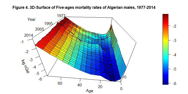
Then, we deduce matrix of the single ages mortality rates using
getqxt() of the $Q2q$ package.
interpolated_surface <- getqxt(Qxt=Bxt, nag=17, t=38)
str(interpolated_surface)
#> List of 8
#>  $ qxt       : num [1:80, 1:38] 0.12771 0.02187 0.01629 0.01181 0.00837 ...
#>   ..- attr(*, "dimnames")=List of 2
#>   .. ..$ : chr [1:80] "0" "1" "2" "3" ...
#>   .. ..$ : NULL
#>  $ lxt       : num [1:81, 1:38] 10000 8723 8532 8393 8294 ...
#>   ..- attr(*, "dimnames")=List of 2
#>   .. ..$ : chr [1:81] "0" "1" "2" "3" ...
#>   .. ..$ : NULL
#>  $ dxt       : num [1:80, 1:38] 1277.1 190.8 139 99.1 69.4 ...
#>   ..- attr(*, "dimnames")=List of 2
#>   .. ..$ : chr [1:80] "0" "1" "2" "3" ...
#>   .. ..$ : NULL
#>  $ qxtk      : num [1:80, 1:38] 0.0587 0.046 0.0353 0.0276 0.0236 ...
#>  $ qxtl      : num [1:70, 1:38] 0.12771 0.02187 0.01629 0.01181 0.00837 ...
#>   ..- attr(*, "dimnames")=List of 2
#>   .. ..$ : chr [1:70] "0" "1" "2" "3" ...
#>   .. ..$ : NULL
#>  $ junct_ages: num [1, 1:38] 16 15 26 62 46 45 28 30 30 29 ...
#>  $ Qxt       : num [1:17, 1:38] 0.1277 0.0571 0.0174 0.0122 0.0132 ...
#>   ..- attr(*, "dimnames")=List of 2
#>   .. ..$ : chr [1:17] "0" "1" "5" "10" ...
#>   .. ..$ : chr [1:38] "X1977" "X1978" "X1979" "X1980" ...
#>  $ Qxt_test  : num [1:17, 1:38] 0.1277 0.0571 0.0174 0.0122 0.0132 ...
#>   ..- attr(*, "dimnames")=List of 2
#>   .. ..$ : chr [1:17] "0" "1" "5" "10" ...
#>   .. ..$ : chr [1:38] "X1977" "X1978" "X1979" "X1980" ...
The obtained result can be represented using a 3D-surface.
par(mar=c(2,2,3,3))
persp3D(x=c(0:79), y=c(1977:2014), z=log(interpolated_surface$qxt), phi = 30, theta = - 175, border = "black", facets = TRUE, inttype = 1, add = F, ticktype = "detailed", expand = .6, scale=1.5, r=.6, box=TRUE, xlab="Age", ylab=NULL, zlab="log nQxt", plot=F, axes=T , main="Figure 5. 3D-Surface of single-ages mortality rates of Algerian males, 1977-2014", cex.main=1 )

text3D(x= 80, y=2010, z= 0.5, labels=c("Year"), add = T, plot=F)
text3D(x= c(84, 82, 82, 79), y=c(1983, 2001, 2008, 2016), z= c(-1.5,-1.5,-1.6,-1.5), labels=c("1977", "1995", "2005", "2014"), add = T)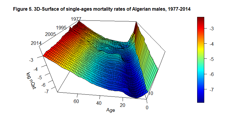
We validate the obtained results using the Fidelity Test and the Zero-One Test:
test_that("Fidelity test", {
 # data("LT")
  Qxt = LT
  expect_equal(getqxt(Qxt, nag=nrow(Qxt), t=ncol(Qxt))$Qxt,getqxt(Qxt, nag=nrow(Qxt), t=ncol(Qxt))$Qxt_test ,tolerance=0.005)
     })
#> Test passed

test_that("Fidelity test", {
  data("LT")
  Qxt = LT
  expect_equal(getqxt(Qxt, nag=nrow(Qxt), t=ncol(Qxt))$Qxt,getqxt(Qxt, nag=nrow(Qxt), t=ncol(Qxt))$Qxt_test ,tolerance=0.005)
   })
#> Test passedLets consider the case of Japanese females in 1950. The dataset can be retrieved from the Japanese Mortality Database , which has a similar structure as the Human Mortality Database and it can be accessed without a prior registration.
library(tidyverse)
#> Warning: le package 'tidyverse' a été compilé avec la version R 4.2.3
#> Warning: le package 'ggplot2' a été compilé avec la version R 4.2.3
#> Warning: le package 'readr' a été compilé avec la version R 4.2.3
#> Warning: le package 'lubridate' a été compilé avec la version R 4.2.3
#> ── Attaching core tidyverse packages ──────────────────────── tidyverse 2.0.0 ──
#> ✔ dplyr     1.1.0     ✔ readr     2.1.4
#> ✔ forcats   1.0.0     ✔ stringr   1.5.0
#> ✔ ggplot2   3.4.3     ✔ tibble    3.1.8
#> ✔ lubridate 1.9.3     ✔ tidyr     1.3.0
#> ✔ purrr     1.0.1
#> ── Conflicts ────────────────────────────────────────── tidyverse_conflicts() ──
#> ✖ readr::edition_get()   masks testthat::edition_get()
#> ✖ dplyr::filter()        masks stats::filter()
#> ✖ purrr::is_null()       masks testthat::is_null()
#> ✖ dplyr::lag()           masks stats::lag()
#> ✖ readr::local_edition() masks testthat::local_edition()
#> ✖ dplyr::matches()       masks tidyr::matches(), testthat::matches()
#> ℹ Use the ]8;;http://conflicted.r-lib.org/conflicted package]8;; to force all conflicts to become errors
# Upload the dataset
LT_3 = read.csv(url("https://www.ipss.go.jp/p-toukei/JMD/00/STATS/fltper_5x1.txt"), sep="", header = F)

# Data manipulation & Preparation
LT_3 = LT_3[-c(1),]
colnames(LT_3) = LT_3[1,]
LT_3 = LT_3[-c(1),]

# Select only the variables of interest (Age and qx)
LT_3 = LT_3 %>% filter(LT_3$Year==1950) %>% select(c(2,4))

# Make sure the dataset is a numerical vector/matrix
m = 19
Qx = as.numeric(LT_3$qx[1:m])

# Plotting the five-age mortality rates
plot(x=c(0,1, seq(5, (length(Qx)-2)*5, by=5)), y=log(Qx), type="b", xlab="Age", ylab="log(nQx)", main="Figure 6. 5-Age Mortality Rates (Japan, females, 1950)", cex=1 ) 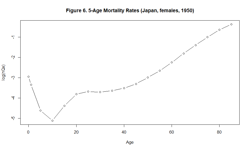
# Interpolating Mortality Rates
qx = getqx(Qx, nag=m)

# Plotting the five-age mortality rates
plot(x=c(0:(5*(m-1)-1)), y=log(qx$qx), type="b", pch=19, xlab="Age", ylab="log(qx)", main="Figure 7. Interpolated Mortality Rates (Japan, females, 1950)", cex=0.75)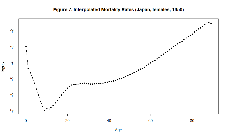
# Results Validation (1): Fidelity Test
test_that("Fidelity test", {
  Qx = Qx
  expect_equal( getqx(Qx, nag=length(Qx))$Qxt, getqx(Qx, nag=length(Qx))$Qxt_test,tolerance=0.005)
   })
#> Test passed

# Results Validation (2): Zero-One Test
test_that("zero-one test", {
  Qx = Qx
  q = getqx(Qx, nag=length(Qx))$qx
  n = nrow(q)
  t = ncol(q)
  expect_true(all(q>0 & q<=1))
})
#> Test passedlibrary(reshape2)
#> Warning: le package 'reshape2' a été compilé avec la version R 4.2.3
#>
#> Attachement du package : 'reshape2'
#> L'objet suivant est masqué depuis 'package:tidyr':
#>
#> smiths
library(tidyverse)
# Upload the data
LT_4 = read.csv(url("https://www.ipss.go.jp/p-toukei/JMD/00/STATS/fltper_5x1.txt"), sep="", header = F)
# Data preparation (Make sure the dataset provided is a numerical matrix)
LT_4_1 = LT_4[-c(1),]
colnames(LT_4_1) = LT_4_1[1,]
LT_4_1 = LT_4_1[-c(1),]
LT_4_1 = LT_4_1 %>% mutate(Age = recode(Age, "0"=0, "1-4"=1,"5-9"=5, "10-14"=10, "15-19"=15, "20-24"=20, "25-29" = 25, "30-34" = 30, "35-39" = 35, "40-44" = 40, "45-49" = 45, "50-54" = 50, "55-59" = 55, "60-64" = 60, "65-69" = 65, "70-74" = 70, "75-79" = 75, "80-84" = 80, "85-89" = 85, "90-94" = 90, "95-99" = 95, "100-104" = 100, "105-109" = 105, "110+" = 110 ))
LT_4_1 = as.data.frame(LT_4_1) %>% mutate(Age=as.numeric(Age), Year = as.numeric(Year), qx=as.numeric(qx))
LT_4_2 = LT_4_1 %>% filter( Year %in% c(1950:1970), Age %in% c(0:85) ) %>% select(Age, Year, qx)
LT_4_2 = dcast(LT_4_2, Age~Year)
#> Using qx as value column: use value.var to override.
rownames(LT_4_2) = LT_4_2$Age
LT_4_2 = LT_4_2 %>% select(-c(Age))
LT_4_2 = as.matrix(LT_4_2)
m = 19
p=21
# Plotting the five-age mortality rates for Japan, females, 1950-1969
library(plot3D)
par(mar=c(2,2,3,3))
persp3D(x=c(0,1, seq(5,85, by=5)), y=c(1950:1970), z=log(LT_4_2), phi = 30, theta = - 175, border = "black", facets = TRUE, inttype = 1, add = F, ticktype = "detailed", expand = .6, scale=1.5, r=.6, box=TRUE, xlab="Age", ylab=NULL, zlab="log nQxt", plot=F, axes=T, main="Figure 8. 3D-Surface of Five-ages mortality rates of Japanese females, 1950-1970", cex.main=1 )
text3D(x= 95, y=1968, z= 0.8, labels=c("Year"), add = T, plot=F)
text3D(x= c(98, 92, 86), y=c(1953, 1963, 1973), z= c(0.15,0.15,0.15), labels=c("1950", "1960", "1970"), add = T)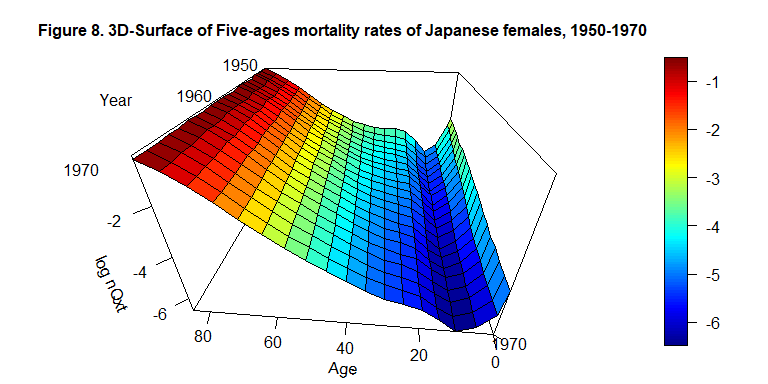
# Interpolating age-specific mortality rates using getqxt function

LT_4_int = getqxt(LT_4_2, nag=19, t=21)

# Plotting the 3D surface of the interpolated mortality rates

library(plot3D)

par(mar=c(2,2,3,3))

persp3D(x=c(0:89), y=c(1950:1970), z=log((LT_4_int$qxt)), phi = 30, theta = - 175, border = "black", facets = TRUE, inttype = 1, add = F, ticktype = "detailed", expand = .6, scale=1.5, r=.6, box=TRUE, xlab="Age", ylab=NULL, zlab="log nQxt", plot=F, axes=T, main="Figure 9. 3D-Surface of age-specific mortality rates of Japanese females, 1950-1970", cex.main=1 )

text3D(x= 95, y=1968, z= 0.8, labels=c("Year"), add = T, plot=F)
text3D(x= c(96, 94, 80), y=c(1959, 1967, 1975), z= c(-0.1,-0.15,0.2), labels=c("1950", "1960", "1970"), add = T)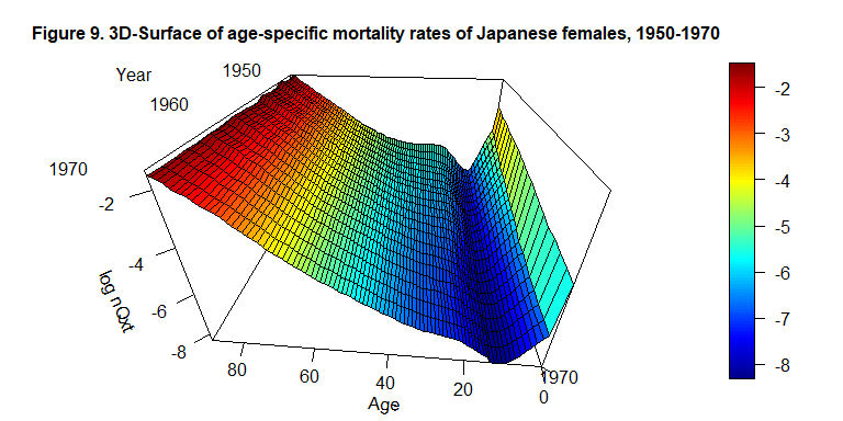
# Results Validation
test_that("Fidelity test", {
  Qxt = LT_4_2
  expect_equal(getqxt(Qxt, nag=nrow(Qxt), t=ncol(Qxt))$Qxt,getqxt(Qxt, nag=nrow(Qxt), t=ncol(Qxt))$Qxt_test ,tolerance=0.005)
     })
#> Test passed

test_that("zero-one test", {
  Qxt = LT_4_2
  q = getqxt(Qxt, nag=nrow(Qxt), t=ncol(Qxt))$qxt
  n = nrow(q)
  t = ncol(q)
  expect_true(all(q>0 & q<=1))
})
#> Test passedShryock, H. S., Siegel, J. S. and Associates (1993). Interpolation: Selected General Methods. In: D. J. Bogue, E. E. Arriaga, D. L. Anderton and G. W. Rumsey (eds), Readings in Population Research Methodology. Vol.1: Basic Tools. Social Development Center/ UN Population Fund, Chicago, pp. 5-48-5-72.